WHAT
Are you prepared to build map legends in a manner keeping with traditional tools and free-range ingredients? Like with locally sourced PNGs and sustainable linear gradient fills? If you’ve never constructed a fine bespoke legend in ArcGIS Pro before, prepare to have the wax blown off your mustache!

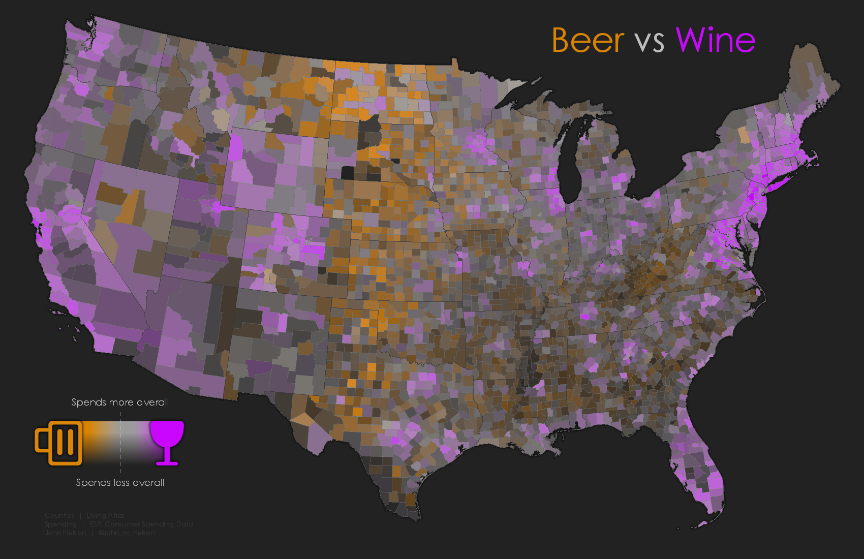
Here is a map of the relative preference of Beer and Wine in US counties. It’s a bivariate map showing 1) a diverging color scheme of orange (strong beer preference) to gray (average comparable preference) to purple (strong wine preference). And atop that is 2) an overlay that suppresses counties that spend less overall, so that higher-booze-spending counties shine through. Here’s how you can make this map, by the way. But I got a lot of questions about the legend…

Now, I’m generally of the opinion that if a map doesn’t need a legend then by all means, don’t give it a legend! But if you must legend a map, there are lots of fun ways to do it. Here is one. It’s a pretty straightforward process, arranging elements in an ArcGIS Pro layout.
HOW
Sometimes you want something a little different than the automated legend generated for you. A map like this is begging for a pictorial legend, and I aim to please. So I grabbed a beer mug icon and a wine goblet icon from the interwebs and I colored them in Adobe Illustrator according to my map; orange for beer and purple for wine. I saved them as transparent PNGs. The transparent bit is important, because otherwise they would have a nasty background and nobody’s got time for that.
This image has fine malty notes and just the right bitter finish. I added both the beer mug and the wine goblet images to the layout via the Insert menu.
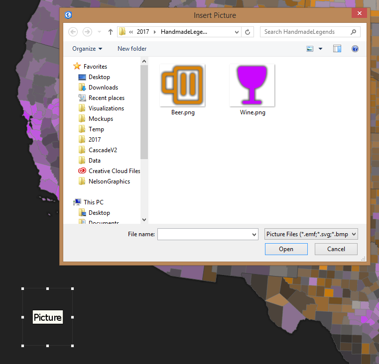
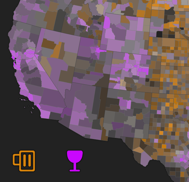
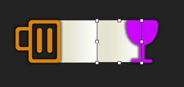
And here they are, both added to the layout. Already I’m digging it. What time is it?
Now to add the linear gradient from orange to gray to purple. I opened up the symbology that paints these values into the counties to check out the colors. Ah the magic of choropleth mapping.
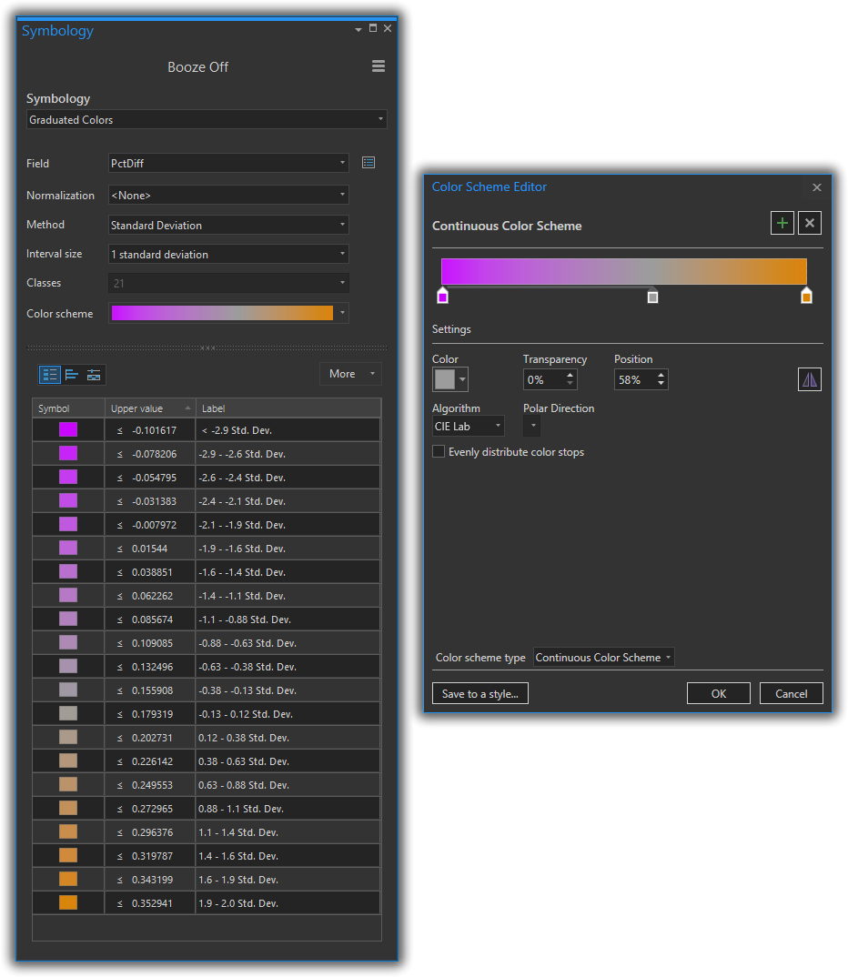
I make note of the three colors my layer is using (I made this color scheme by expanding the droplist of colors and choosing “Format color scheme”). I’ll use these to colorize some rectangles I’m about to drop in behind the images.
I added two rectangles between the cup images. One spanning from under the beer mug to the center and another from the center to the wine goblet.
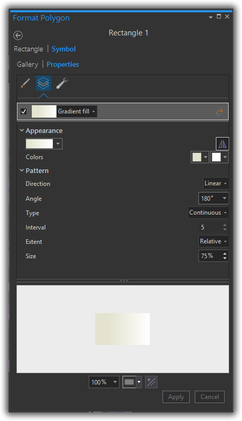
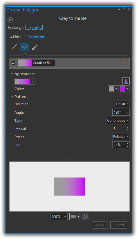
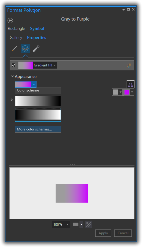
In the rectangle’s format menu (double-click the rectangle) you can set the fill to be a gradient. I tweaked the settings until I got a continuous horizontal gradient from one color to another. I did this for both the beer and wine rectangles. I added two rectangles, and gradients, to replicate the map layer’s diverging gradient with three stops (the standard color options only provide two options).
Before setting the colors…
After setting the colors…
—
Pro tip (wink): If I had saved this map layer’s color gradient as a style, I could just pick it from a list. As Edie Punt says, “styles are your friend.” And I agree. Here’s where to choose from your set of saved styles, if you go this route. Expand the “appearance” droplist, and choose “More color schemes.” You’ll see your delicious saved styles there.
—
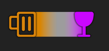
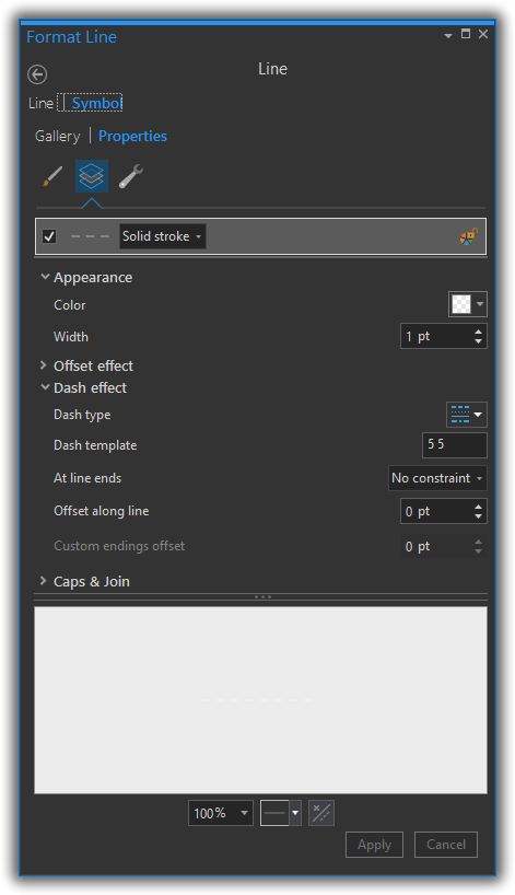
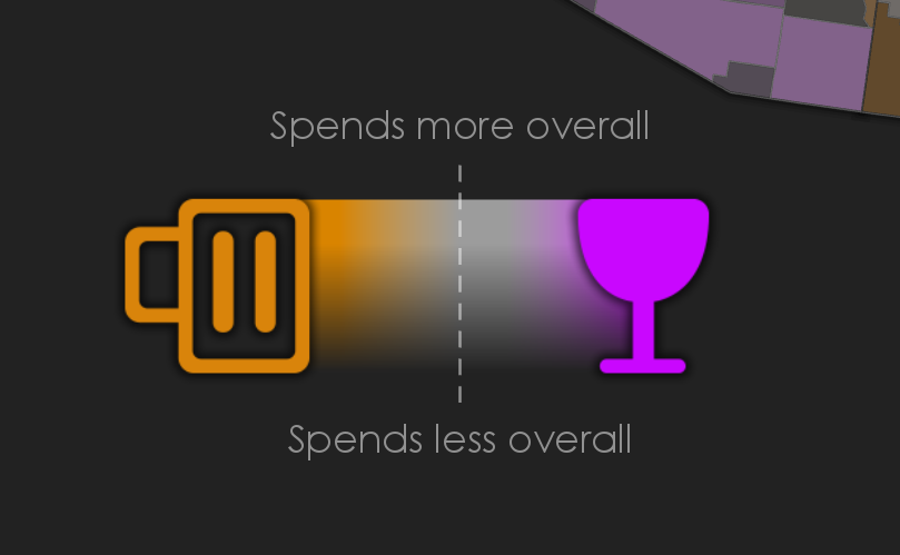
Cool! These two rectangles look like a single three-part gradient spanning image to image (I didn’t use the sneaky saved style trick). Next, I thought it would be nice to add a faint dashed line in the middle, denoting the average. This is just a line, inserted and formatted to be dashed.

The dashed line format looks like this…
But what about the whole “bivariate” nature of this thing? So far, this legend only shows the linear transition from beer preference to wine preference. The map also includes the dimension of overall spending, to help normalize this thing and provide a more nuanced surface of booze spending.
No problem! The map uses a copy of the counties layer that uses the background color and transitions from more opaque in low-spending counties to more transparent in high-spending counties. This way, higher spending colors shine through more while lower spending counties recede. It’s a nice hack -used a lot on election maps to normalize by population.
I just do the same exact thing with the legend. On top of the rectangles that illustrate the color gradient of beer/wine preference, I plop in a rectangle with a vertical (up and down) gradient that transitions from a fully transparent version of the map’s dark gray background color down to fully opaque version of the background color.
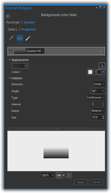
Which looks like this…
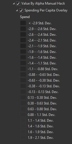
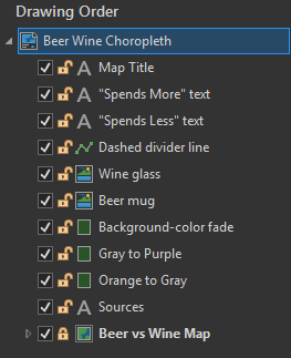
This, for reference, is what the Layout Contents panel looks like, to provide a sense of the elements and their layering…
So there it is! A hand-crafted fine fine artisanal bespoke legend. Ready to inform and delight your map readers of the rich intricacies of your maps.
WHAT??
Once you get comfortable using the picture and drawing elements in your map layout, you are capable of all sorts of shenanigans. For example, there’s no reason you have to stick with color and opacity to denote your bivariate map. Maybe you instead want to live dangerously and use Chernoff faces to illustrate beer/wine preference and spending…
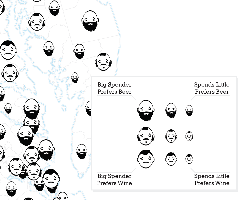
What?? Chernoff faces in ArcGIS Pro?! Yes, it ain’t no thang. Once you have a bevvy of symbol assets, you can make all sorts of Chernoff trouble. But I’m getting ahead of myself.
Happy Legending! John

Article Discussion: