Since this article was written, some enhancements were made in ArcGIS Pro to make simplify the user experience and integrate this with other part of the software such as time and range sliders.
Please read the following blogs that talks about this in greater details.
- Dynamic Spatiotemporal Exploratory Analysis with Aggregated Results Using Time Series Data in ArcGIS
- Transform Dynamically Aggregated Time Series Results into Polygons in ArcGIS
- Dynamic Aggregate Points within Polygon Features for Exploratory Analysis
- Play back flight data using time slider and query layer in ArcGIS Pro
Time-series data stores observations, measurements, model results, or other data obtained over a period of time, at regular or irregular intervals. They can be broadly classified into two groups:
One where the location of an entity moves over the time, e.g. vehicle tracking etc.
Another one is where locations are stationary but v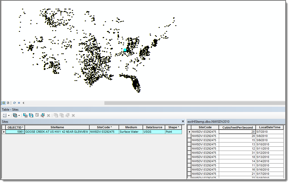 alues are measured over time at those locations. For example, temperature and wind speeds are collected at weather stations on a daily basis, or water flow or quality may be measured at gauges along streams at irregular intervals. In these examples, weather stations and gauges along streams are stationary (their locations do not change) while observed data such as temperature, wind speed, or water quality etc. that change over time are dynamic.
The later case is the focus of this blog post.
To maintain it efficiently in a geodatabase, this information is stored in two separate tables. One is a spatial table that contains locations, unique identifiers and may have some descriptive attributes such as name, type etc. And a second table stores observed data, the date time when observation was made, and an identifier to link the data to location stored in the spatial table. The spatial table will be referred to as an “asset table” and the second table will be referred to as an “observation table” in this blog. There is basically a one-to-many relationship between these two tables – that means for one location in the asset table, there are multiple records in the observation table.
Since the introduction of time-aware layers in ArcGIS 10.0, you can display features with time-series data from 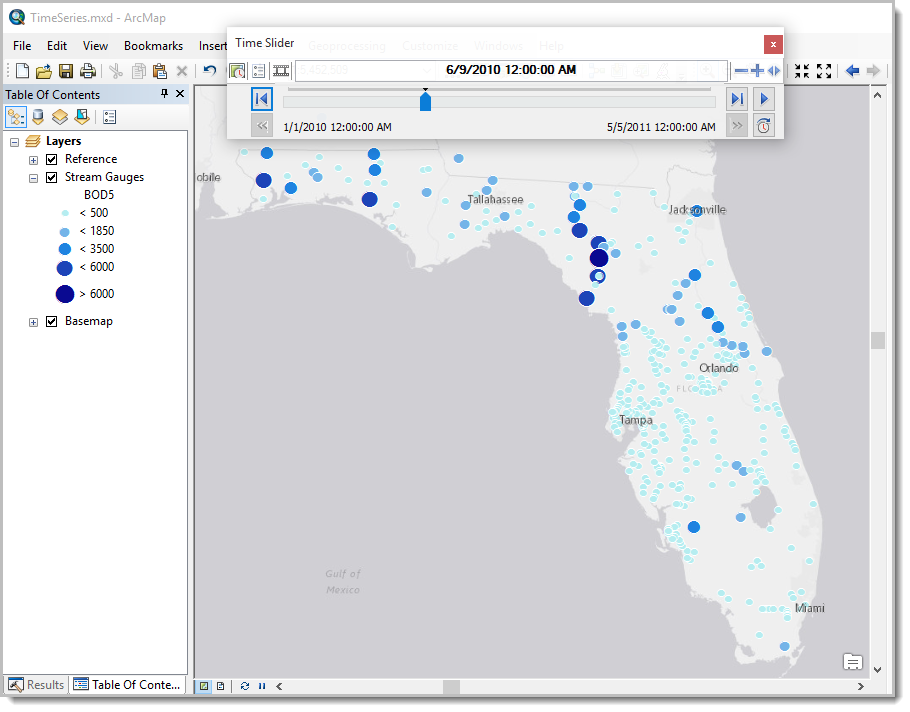 a separate table, collected at regular intervals with one additional step. This allows you, using the time slider, to go back in time and draw features with the observed or measured values for a given time instance.
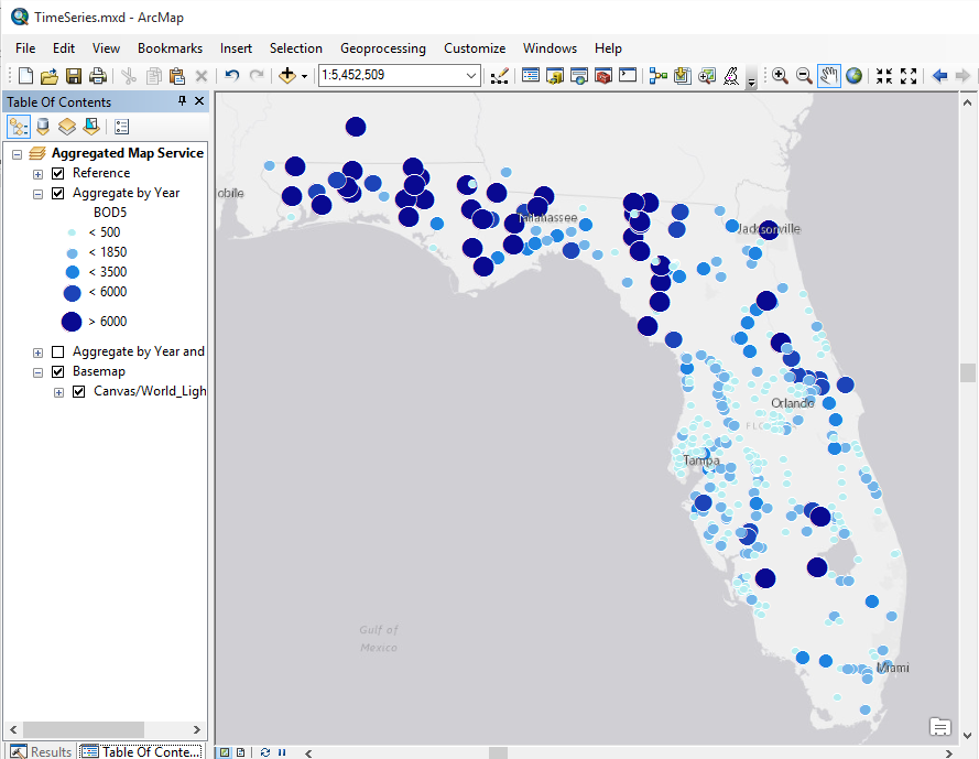
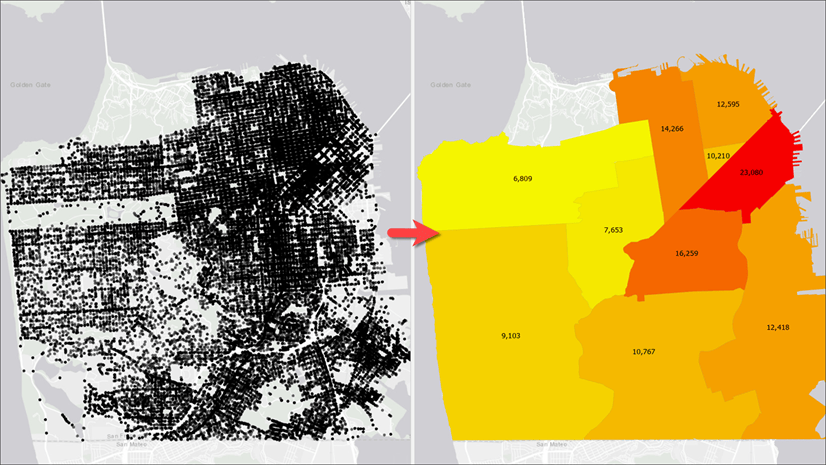
That is great, but sometimes for various analytical reasons, you need to display features using some summary statistics – instead of raw observed data – for a given time duration. For example, you may want to map weather stations with monthly average temperatures for January 2016 from an observation table where daily data was stored. Another reason you may want to display features with summary statistics is to discover patterns — especially from a time-series data observed at irregular intervals which otherwise would not be possible.
To make matters more complicated, there are cases where the asset and observation tables are stored in a single database and in other cases they are stored in separate databases. For the best performance, it is always recommended to keep asset and observation tables in the same database.
In this post, I will describe what you need to do:
- To create layers to display features with aggregated results that get computed on the fly.
- Use a definition query to show results only for a predefined time window.
- To author and publish a map service.
- Build a web application using an existing application template to consume the map service to be used by your end users.
In another post, if you feel adventurous, I will discuss how you can write custom code to achieve the same goal but with a better user experience using the time slider. Here is the link to that post.
Notes
- Your data needs to be in an enterprise database such as SQL Server, Oracle, PostreSQL or Netezza. A file geodatabase or other file-based data sources will not work.
- All SQL expressions are provided here to retrieve date parts that are specific to SQL Server. If you are not using SQL Server, please consult your database documentation.
Create Layer to aggregate results for a predefined time window
Add layer
This section tells you steps what to do when asset and observation tables are stored in the same database. If these tables are stored in separate databases, please skip this section and go to the “What to do when tables are stored in separate databases” section below.
- In ArcMap, open the New Query Layer dialog box: File > Add Data > Add Query Layer.
- Select an existing database connection from the Connection drop-down box, or create a new one by clicking the Connections button.
- Type a name (e.g., “Aggregate by year”).
- Type the following SQL query in the Query text box:
SELECT a.OBJECTID, a.Shape, o.* FROM AssetTable AS a
 INNER JOIN
  (SELECT Station_ID,
     (DATEPART(YEAR, [localdatetime])) AS compyear,
     MIN(MeasuredValue) AS min_MeasuredValue,
     MAX(MeasuredValue) AS max_MeasuredValue,
     AVG(MeasuredValue) AS avg_MeasuredValue
   FROM ObservationTable
   GROUP BY Station_ID,
     (DATEPART(YEAR, [localdatetime]))
  ) AS o
 ON a.Station_ID = o.Station_ID
The above query is to return the yearly aggregated result. Here are SQL queries if you need to retrieve monthly aggregated results:
SELECT a.OBJECTID, a.Shape, o.* FROM AssetTable AS a
 INNER JOIN
  (SELECT Station_ID,
     (DATEPART(YEAR, [localdatetime])) AS compyear,
     (DATEPART(MONTH, [localdatetime])) AS compmonth,
     MIN(MeasuredValue) AS min_MeasuredValue,
     MAX(MeasuredValue) AS max_MeasuredValue,
     AVG(MeasuredValue) AS avg_MeasuredValue
   FROM ObservationTable
   GROUP BY Station_ID,
     (DATEPART(YEAR, [localdatetime])),
     (DATEPART(MONTH, [localdatetime]))
  ) AS o
 ON a.Station_ID = o.Station_ID
or daily aggregated results:
SELECT a.OBJECTID, a.Shape, o.* FROM AssetTable AS a INNER JOIN (SELECT Station_ID, (DATEPART(YEAR, [localdatetime])) AS compyear, (DATEPART(MONTH, [localdatetime])) AS compmonth, (DATEPART(DAY, [localdatetime])) AS compmonth, MIN(MeasuredValue) AS min_MeasuredValue, MAX(MeasuredValue) AS max_MeasuredValue, AVG(MeasuredValue) AS avg_MeasuredValue FROM ObservationTable GROUP BY Station_ID, (DATEPART(YEAR, [localdatetime])), (DATEPART(MONTH, [localdatetime])), (DATEPART(DAY, [localdatetime])) ) AS o ON a.Station_ID = o.Station_ID - Click the Validate button.
- Click Next.
- Make sure the ObjectID field, geometry type, and spatial reference that got picked automatically are correct.
- Click OK to add the layer with aggregated results in its attribute table.
- Following the steps above, create another query layer using the SQL expression (provided above) to show the monthly aggregate results.
Setting layer properties
Both of these layers are showing multiple points for the same location, since the aggregated result is grouped by year and joined to the asset table. Use the definition query to show results for only one year or one month.
- Open the first layer’s property page and click the Definition Query tab.
- Add a query (e.g., COMPYEAR = 2015) to show only results for 2015.
- Click the Apply button.
- Click Symbology tab.
- Select Graduated Colors or Graduated Symbols.
- Select one of those aggregated fields (e.g., Max_MeasuredValue, Min_MeasuredValue or Avg_MeasuredValue).
- Classify and symbolize as you prefer.
- Click OK to draw.
- Repeat these steps for the second layer but with a minor difference: you need to use two fields in the definition query (i.e., COMPYEAR = 2015 AND COMPMONTH = 1) to show results for January 2015. If you want to have a third layer to show daily aggregated result, use three fields (i.e. COMPYEAR, COMPMONTH, and COMPDAY) in the definition query.
Share as a map service
Next logical step is to share the layers as a map service to make it easily accessible by others. This section talks about what needs to be considered before publishing these layers as a map service.
- Open the layer property page and remove the existing definition query.
That is because the REST API for Map Services does not allow you to override a layer’s existing definition queries. - Make the layer invisible.
If you don’t do that and the layer does not have any definition query, the layer draws the same features multiple times and the request that goes to the database performs a full table scan. This is not desirable and may even overload the underlying database especially when the observation table contains millions of records. - Go to File > Share As > Service to start the publishing process.
- Follow the wizard; once the Service Editor dialog appears, select Mapping from the left panel and check Allow per request modification of layer order and symbology.
This will allow a web application to modify the layer’s symbology and renderer. - Click the Analyze button, check the Prepare window and make sure there are no unexpected warnings. If you see the message Data source is not registered with the server, right-click it and select the Register Data Source With Server option (you must not copy your data to the server).
- Click Publish button from the upper right corner to create a map service.
Create and share a web application
Since viewing aggregated results for any given time window requires the end users to set filter or definition query from the web application, we need do some extra steps to make sure that there is always a default filter or definition query set to each sublayer within the map service layer.
Create a web map and set default filter
- Open ArcGIS Online or Portal Map Viewer on a web browser.
- Add the map service you published earlier to the Map Viewer.
- Expand the layer on the map’s Contents pane to show its sublayers.
- Point to the first sublayer and click the Filter button.
- Set the filter to COMPYEAR = 2015.
- Make sure to check the Ask for values check box and fill up the Prompt and Hint textboxes so that your end users can’t view the map service without the definition query and won’t overload the database.
- Click Apply Filter.
- Make the sublayer visible from the Contents pane.
Now you are seeing features drawn with the type of aggregation you chose while preparing the layer for the year 2015 in ArcMap. - Alternatively, if you want to change the symbol styles or view using a different aggregation method, point to the sublayer and click the Style button.
- Choose one of the fields with aggregated results (e.g., Max_MeasuredValue, Min_MeasuredValue, or Avg_MeasuredValue).
- Select a drawing style and click Done.
- Following the above steps, set a filter for the second sublayer. Please note: You need to use both COMPYEAR and COMPMONTH in the filter – you need to add two expressions in the Filter dialog and make sure Ask for values is checked for both expressions.
- Save the map.
Create a web application using an existing application template
- Still on the Map Viewer, click the Share button.
- On the Share dialog box, click the Create a Web App option.
- Search for application templates with the “filter” keyword.
- From the search result choose the template named Filter.
- Click Create App and fill in the necessary boxes in the next dialog box.
- Click Done which brings up the Configure Web App page.
- Select Filter Options and check Display dropdown.
- Click the Save and View button close the configuration pane and open the web application.
You can share this web application with your end users. While using this application, to view the aggregated result for a given period, select the layer from the drop-down menu, modify the filter, and click Apply.

What to do when tables are stored in separate databases
There are some cases where the observation table is stored in a separate database, which you can only connect to using ODBC/OLE DB drivers from ArcGIS. This procedure involves additional steps and may require some database knowledge and privileges.
Note: Make sure a 64 bit version of your OLE DB/ODBC drivers are installed on the server machine(s).
Create views in the database
- Connect to your database using a database client application. For example for SQL Server, you can use SQL Server Management Studio.
- Create a view to aggregate results by year.
SELECT Station_ID,
	(DATEPART(YEAR, [localdatetime])) AS compyear,
	MIN(CubicFeetPerSecond) AS Min_MeasuredValue,
	MAX(CubicFeetPerSecond) AS Max_MeasuredValue,
	AVG(CubicFeetPerSecond) AS Avg_MeasuredValue
	FROM ObservationTable
	GROUP BY Station_ID,
		 (DATEPART(YEAR, [localdatetime]))
- Create a second view to aggregate results by month.
SELECT Station_ID,
	(DATEPART(YEAR, [localdatetime])) AS compyear,
	(DATEPART(MONTH,[localdatetime])) AS compmonth,
	MIN(CubicFeetPerSecond) AS Min_MeasuredValue,
	MAX(CubicFeetPerSecond) AS Max_MeasuredValue,
	AVG(CubicFeetPerSecond) AS Avg_MeasuredValue
	FROM ObservationTable
	GROUP BY Station_ID,
		(DATEPART(YEAR, [localdatetime])),
		(DATEPART(MONTH, [localdatetime]))
Create an OLE DB connection in ArcCatalog
- Open ArcCatalog.
- Click Customize Mode from the Customize menu.
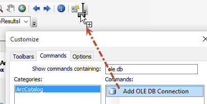
- Click the Commands tab on the Customize dialog box.
- Type OLE DB in the Show commands containing box.

- Drag the Add OLE DB Connection command onto any toolbar.
- Close the Customize dialog box.
- Click the newly added Add OLE DB Connection button to bring up the Data Link Properties dialog.
- Fill in the dialog to create a connection to your database.
- The newly created connection will show up under the Database Connections node in the Catalog window in both ArcCatalog and ArcMap.
Add layers in ArcMap
- In the ArcMap Catalog window, expand the Database Connections node, and find the connection you created in the previous step, and double-click to connect.
- Find the views you created earlier and add them to the map.
- Connect to your enterprise geodatabase where the asset feature class is stored.
- Add the asset feature class to the map.
- Open the layer’s property page and click the Joins and Relates tab.
- Create a join to the table that is for yearly aggregation.
- Add the asset feature class to the map again.
- Open the layer’s property page and click the Joins and Relates tab.
- Create a join to the table that is for monthly aggregation.
Performance tips:
For best performance, make sure that
- The primary and foreign fields that are used to create the join between the asset and observation tables are indexed.
- The time field is indexed as well.
- Create indexes for the SQL expressions (i.e., DatePart() ) you used earlier in SQL queries.
Please note: SQL Server requires you to add non-persisted-computed fields using those expressions to the observation table, then create indexes on them and use those computed name in the definitions of the views or query layers instead of using expressions.
Dynamically computing aggregated values has merits – you always see results from the latest set of data. But there is a performance hit, since aggregated results are computed on the fly. If you don’t need to compute those values dynamically, you can precompute them and/or have some kind of task that can be scheduled to run at regular intervals to update those precomputed values with the latest data. If you choose to do this, you don’t need to use SQL expressions while creating the query layer; instead, just use the precomputed fields.
Contributed by Nawajish Noman, Craig Williams and Tim Ormsby of the ArcGIS development team.

Article Discussion: