Prepare the Data
In part 1 of this blog, we showed you how to take species observation data such as museum records with an x, y coordinate pair and drag and drop it into ArcGIS.com map to make a web map. We used data we downloaded from the Fishnet website to make a web mapping application showing records for Speckled Dace.
Let’s say you click on a point in this map, what do you see? You see a simple list of attributes. It’s a start. But you have to scroll way down to see the important things like the collection date and the collector. Other values could use some clean up on the database side to make the map more presentable. For example, values for counties include “Benton County”, “Catron”, “DOUGLAS” and “Kittitas Co.” while other records have no value for county at all.
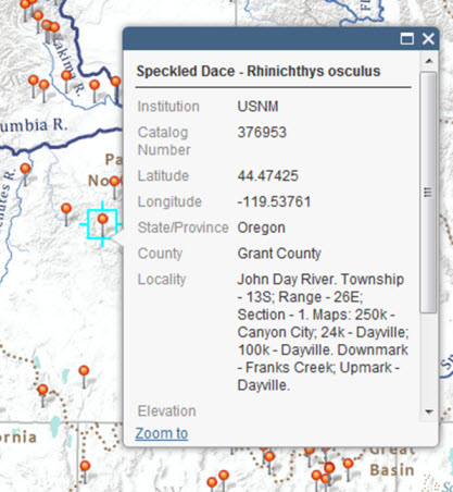
Figure 1: The original pop-up window from our Speckled Dace map.
In version 2.0 of our Speckled Dace map we used the field calculator in ArcMap to format the data a bit first before it goes into a pop-up window. To build this new map we downloaded the most recent version of the Fishnet query for Rhinichthys osculus and deleted records without coordinates. These data records sometimes contain commas in their fields, so we chose to download the tab-delimited format, *.txt. We imported the table to a geodatabase and added it to a new ArcMap document for editing.
Specimen
The catalog number and museum code are used to refer to a particular specimen held by a specific institution in scientific publications. The catalog number is the key value that unlocks all sorts of information about a specimen, including notes kept by the collector and other related information.
The original pop-up displayed the institution and catalog number separately because they are in two different fields. We think our map reader would like to see them together because they make more sense to our audience when read together like this:
UWFC 029568
The CatalogNumber field in the Speckled Dace dataset contains a variety of data: numbers, text plus numbers, and combinations of text, numbers and special characters. A second field, InstitutionCode, is relatively straightforward. InstitutionCode provides the standard code used to identify the museum that owns the specimen. This field is fully populated and needs no modification.
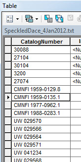
Figure 2: Data in the CatalogNumber field are in different formats and need to be standardized for the pop-up.
To standardize the catalog number we first added a new field, CatNum, to the table as text format field and set its length to 20.
As we mentioned the CatalogNumber field has data formatted different ways, including some records with their museum codes still attached. To remove the museum codes from the catalog numbers first right-click the CatNum field and then select field calculator. Then we use a simple Python function to split the CatalogNumber field and populate the CatNum field with the museum code removed.
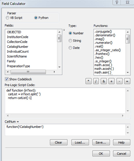
Figure 3: Screen shot of the field calculator with Split_CatalogNumber.cal calculation file loaded.
Note that the python parser radio button has been selected and there are two windows into which to place code, the pre-logic script code window, and the window below it where the field calculation is defined. Be sure when you do your calculation to check the Show Codeblock box, otherwise you will not see the pre-logic script code window.
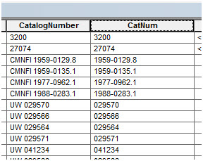
Figure 4: The data table after performing the calculation using the Split_CatalogNumber.cal calculation file.
CatNum is now populated with the catalog number of each specimen and its museum code removed.
We would like to provide a link from each record to the web page of the institution that provided the data. We can do that by joining a table of with hyperlinks in it to our original table. To add links we made a new table with fields that will contain the museum codes and hyperlinks.
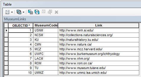
Figure 5: Lookup table for adding links to museum web pages.
Join the museum links table to the fishnet records using InstitutionCode field from the original table and MuseumCode from the museum link table. Next, export the joined table to make the join permanent. The extra MuseumCode and OBJECTID_1 fields may be deleted from the new table.
We then made a new text field, Specimen, and set its length to 200. To create this field we will use field calculator (Specimen_html.cal) to merge the InstitutionCode, CatNum, and Link fields and add a hyperlink.
The Specimen_html.cal calculation file does not use a python function so it only has the following code in the field calculation window:
“<a href=”” + !Link! + “”> ” + !InstitutionCode! + “</a> ” + !CatNum!
This concatenates the InstitutionCode, CatNum, and Link fields and adds a hyperlink with an HTML link tag.
The new Specimen field is populated with values that look like this:
<a href=”http://www.museum.tulane.edu/”> TU</a> 93821
Because ArcGIS.com understands the meaning of the HTML link tag, the field will display in the pop-up like this:
TU 93821
The museum code is now linked to the museum’s webpage! The specimen field is now ready for the web map. Once this is all working properly you can place hyperlinks in your arcgis.com map pop-ups and have all kinds of information available to your map viewer without the needless clutter of dumping things unformatted into the pop-up window.
Locality
In the original version of the Speckled Dace map, information about location of the record was split amongst three fields, StateProvince, County, and Locality.
Raw values in the StateProvince field are both capitalized and un-capitalized. We could run a simple capitalization script, however some states such as North Dakota and New Mexico have two words in their names that need to be capitalized, so we recommend using a script to calculate this field so that everything comes out the way it should. This script is called State_caps.cal and is the following:
State_caps.cal
Pre-logic Script Code:
def function(State):
final = “”
split = State.split()
for word in split:
caps = word.capitalize()
final += caps + ” ”
final = final.strip()
return final
Field Calculation:
StateProvince = function(!StateProvince!)
To run the calculation script we right-clicked the StateProvince field, selected field calculator, loaded and then ran the State_caps.cal script.
Counties are even more complicated, some values end in “Co.” while others end in “county”. Still others are in Canada where the county field is not populated. The following County_Cleanup.cal script traps all these cases and standardizes the field:
County_Cleanup.cal
Pre-logic Script Code:
def function(county, state):
if county[-3:] == “Co.”:
return county[:-3] + ” County”
else:
if county.find(“County”) == -1 and state != “British Columbia”:
return county + ” County”
else:
return county
Field Calculation:
County = function(!County!, !StateProvince!)
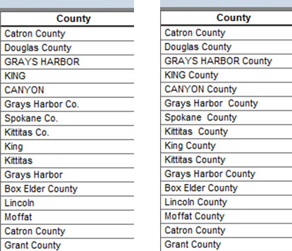
Figure 6: The County field before and after running the County_Cleanup.cal script. Note that the counties still have irregular capitalization.
The last step for preparing the counties is to standardize capitalization. To do this we ran the County_caps.cal script which is very similar to the State_caps.cal script.
County_caps.cal
Pre-Logic Script Code:
def function(CountyCap):
final = “”
split = CountyCap.split()
for word in split:
caps = word.capitalize()
final += caps + ” ”
final = final.strip()
return final
Field Calculation:
County = function( !County! )
To standardize the capitalization we used a second script (County_caps.cal) that is similar to the one used to fix the capitalization of the StateProvince field.
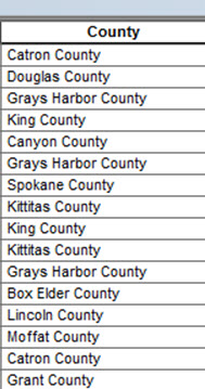
Figure 7: Final County field ready for use in web map.
To organize the locality information contained in the StateProvince, County, and Locality fields into a single field we first need to tackle the case of records with no locality data. First we sorted the table so the fields with NULL values in their locality field are all in a row. Then we highlighted these records and used field calculator to populate them with the value “x” which a later script will change into “No locality information reported.”
We then cleared the selection and added a text field LocHTML and set its length to 250. We ran a field calculator script (Locality.cal) to assemble the three fields for the web map.
Locality.cal
Pre-logic Script Code:
def function(loc):
length = len(loc)
if length > 200:
loc = loc[:200] + “…”
else:
if loc[-1:] != “.”:
loc = loc + “.”
return loc
def countyFunction(county):
if county == “x”:
county = ” ”
else:
county = ” ” + county + “, ”
return county
Field Calculation:
function( !Locality! ) + countyFunction(!County!) + ( !StateProvince!) + “.”
Because fields in a dbf file cannot be longer than 254 characters, the Locality.cal script trims Locality values greater than 200 characters, leaving space for the county and state. If the locality is clipped an ellipsis is added (“…”) to indicate that more information is associated with the original record. Next if the Locality does not end in a period one is added. If the County field is = “x” a space is added to the end of the locality string otherwise a space followed by the County value then a comma and space are appended to the locality string. Lastly the state and a period are added yielding values that look like this:
New Fork River 1.5 mi. W of Pinedale, US Hwy. 187. Sublette County, Wyoming.
No locality information reported. Idaho.
North Fork John Day River. Oregon.
Collection Date
In our original map the collection date is displayed in three rows, in a number format. Because using a number for the month can be confusing to international audiences, we wanted to convert the MonthCollected field to a text field instead of a number field.
First we made a lookup table which contains the name of each month and the number of each month in two fields. We are going to concatenate some of these fields together, so we need to limit the lengths of each of the fields for right now. The Month field should be an integer, and the MonthText field should be a text field with a length of 40.
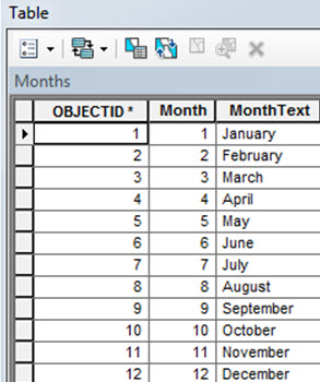
Figure 8: Lookup table used to convert MonthCollected values from number to text.
We then joined the new table’s Month field to the original tables MonthCollected field. We exported the joined table to make the join permanent and then deleted the Month and OBJECTID_1 fields. We sorted the new table on the MonthText field and select null values. We used the field calculator to set the null values to “Collection date not provided” (this is why we made the field length = 40).
We then added a new text field named Full_Date to the table and set its length to 40. We used the field calculator script Date.cal to assemble the month, day, and year for the web map.
Date.cal
Pre-logic Script Code:
def function(month, day, year):
if month == “None”:
date = “Collection date not provided”
else:
date = month + ” ” + str(day) + “, ” + str(year)
return date
Field Calculation:
function( !MonthText! , !DayCollected! , !YearCollected! )
Collector
We sorted the Collector field and selected the null values. We then used the field calculator to set the null values to “Unknown”.
Now the data are ready for use in our web map. Right click the table in ArcMap and export the table to a text file (*.txt).
Next week
Next week we will show you how to configure a custom pop-up format that we used to make our new speckled dace web application.
Download the Field Calculator Scripts
We posted the field calculation scripts on the ArcGIS Hydro Resource Center for you to download, use, and modify.
County_caps.cal
County_Cleanup.cal
Date.cal
Locality.cal
Specimen_html.cal
Split_CatalogNumber.cal
State_caps.cal
Special Thanks to:
The Fishnet data portal data portal and the following institutions for providing the data used in this application:
- US National Museum of Natural History
- North Carolina Museum of Natural Sciences
- University of Kansas Natural History Museum
- Canadian Museum of Nature
- Harvard University Museum of Comparative Zoology
- University of Washington Fish Collection
- Natural History Museum Los Angeles County
- Royal Ontario Museum
- Tulane University Museum of Natural History
- University of Michigan Museum of Zoology
And to Rich Nauman and Michael Dangermond for providing the post. For more information on using biodiversity data in ArcGIS.com web maps and applications contact Richard Nauman (rnauman@esri.com).

Article Discussion: