By Rajinder Nagi, Esri Cartographic Product Engineer
![]()
A common cartographic technique is to transparently overlay a colored raster, called a layer tint, over a grayscale raster, like a hillshade or a panchromatic aerial or satellite image. When you display a colored raster transparently over a grayscale raster, you lose the intensity of your colors and that it is harder to see the hillshade details.
In this blog entry, we explain how you can overlay colored rasters on grayscale rasters without losing detail in the graytones or intensity in the colors. The example here uses color ramps and Image Analysis functions. In a related blog entry, we demonstrate the same overlay method using colorramp files and mosaic dataset functions. No matter how you work with your rasters, this new overlay method will allow you to retain the detail and colors in the overlaid rasters.
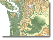
In the example below, a layer tint with colors that relate to elevation values (figure 1) is overlaid on a gray hillshade of the land surface (figure 2).

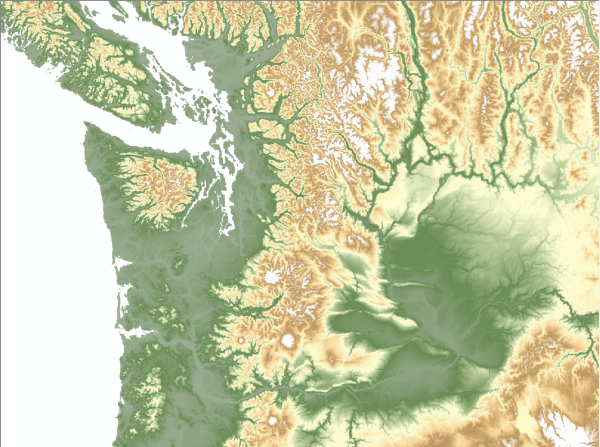
Figure 1. A layer tint of elevation

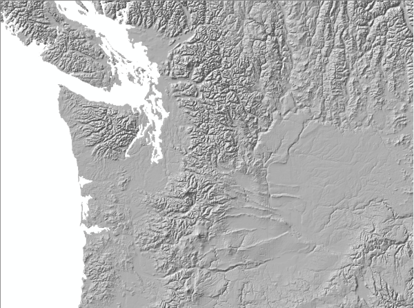
Figure 2. A grayscale hillshade
This results in a display that has a washed-out version of the layer tint and a less detailed version of the grayscale raster (figure 3).

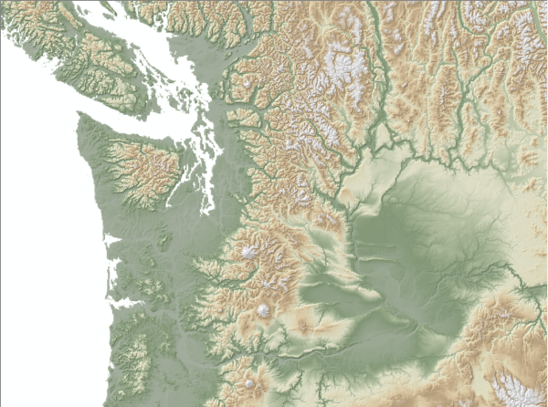
Figure 3. The result when the layer tint is shown with 40 percent transparency over the hillshade
In this blog post, we describe how to obtain the results in figure 4 by using a color ramp and Image Analyst functions to retain both the original colors and the grayscale detail in the input rasters.

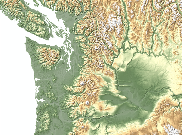
Figure 4. The result when image functions are used to control the display
At the core of this display method is a combination of pan-sharpening, contrast stretching, and gamma stretching functions. The pan-sharpening function uses a panchromatic and a multispectral (three-band RGB) raster as input. In the example here, the inputs are (1) a hillshade created from a DEM as the panchromatic raster and (2) a DEM with a color ramp that has been converted to a multispectral raster. The output from the pan-sharpening function is then used as input for the contrast and gamma stretching functions.
Since layer-tinted DEMs are not usually managed as three-band RGB rasters, a conversion is required. To do this, add the DEM to ArcMap, right-click the layer in the table of contents, and click Properties. On the Symbology tab, select the color ramp you want to use to display the data. Click OK to close the Layer Properties dialog box. Right-click the layer in the table of contents, click Data, and click Export Data. In the Export Raster Data dialog box, check Use Renderer and check Force RGB. Choose a location and input a name, then click Save. Choose to add the exported data to the map as a layer. The three-band RGB image will be added to the table of contents.
At this point, you can either follow the steps described in the previous article to add the raster to a mosaic dataset and render it, or you can use the instructions below if you want to use the Image Analysis tools instead of a mosaic dataset.
Define the functions for the raster datasets by following the steps below:
1. Add the grayscale hillshade and multispectral RGB layer tint rasters to ArcMap, if they have not already been added.
2. Open the Image Analysis window by clicking Windows on the top bar menu, then clicking Image Analysis.
3. In the top section of the Image Analysis window, select both the hillshade and RGB rasters using the Control key and clicking on each raster’s name to highlight it (figure 5).

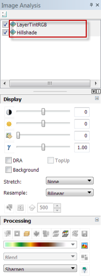
Figure 5. The Image Analysis window
4. Click the Pan-Sharpening tool in the Processing section of the Image Analysis window. This will create a new layer, which will be listed as the top layer in the Image Analysis window.
5. In the Image Analysis window, right-click the newly generated pan-sharpening layer and click Properties.
6. On the Functions tab, right-click the Pansharpening Function and click Properties.
7. On the General tab of the Raster Function Properties dialog box, change the Output Pixel Type to 8 Bit Unsigned.
8. On the Pan Sharpen tab, change the Method to Simple Mean.
9. Keep the rest of the defaults and click OK.
10. Right-click Pansharpening Function, click Insert, and click Stretch Function.
11. Change the Type to Minimum-Maximum.
12. Check the Use Gamma option.
13. In the Gamma section of the dialog box, change the Gamma value from 1.0 to 0.5 for each of the three bands.
14. In the Statistics section of the dialog box, type 5 as the Min and 215 as the Max value for each of the three bands. The final function chain will look like figure 6.

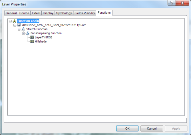
Figure 6. The final function chain
15. Click OK to check your results.
After checking the results, feel free to experiment with the gamma, minimum, and maximum values in the Stretch Function.
Creating your display by using the Image Analysis window instead of mosaic datasets results in a temporary raster. If you want to keep your results, export the layer that you added the functions to from ArcMap. To do this, right-click the layer in the table of contents and click Export Data. The data you save can now be added to an ArcMap session and will display with the final results.
If you want to try this out yourself, download this .zip file which contains a map package of the Washington elevation map used in this article.
Thanks to Aileen Buckley, Mapping Center Lead, for her help with this blog entry!

Rajinder,
Wonderful article! I’ve been using the semi-transparent method for years but have been disappointed with the results. Where can we find the hillshade used in the article?
Thank you,
Randy
Thanks for your comment! Give it a try and I hope you will like it. I created the hillshade in this example from GTOPO30 DEM, which is freely available to download from USGS site here: http://eros.usgs.gov/#/Find_Data/Products_and_Data_Available/gtopo30_info.
I added a link at the end of the blog post to a zip file that you can download that has the map document used to create the graphics for this article.
All too often, the workflow from these “how to’s” end up creating yet ANOTHER dataset that you have to maintain and allocate disk space for. Why would you do this when you can achieve the same effect illustrated in this blog post by simply increasing the brightness and contrast values for your hillshade raster? I doubt the differences between my suggestion and your technique would really be noticable.
Raster Functions are not only fast, efficient, and powerful, but they also do not take up any additional space on your hard disk. Raster Functions are performed on-the-fly, therefore you are not spending time writing out a file or taking up additional space. Raster functions can be stacked up (as Rajinder has shown), so you can perform multiple processes on your layer(s).
To read more on raster functions, you can visit the following URL:
http://help.arcgis.com/en/arcgisdesktop/10.0/help/index.html#/Rasters_with_functions/009t0000000m000000/
@evtguy
If you don’t want to create another dataset, then use Mosaic dataset option I described in my previous article here: http://goo.gl/bnsD4
Mosaic datasets store pointers to the physical data on the disk and don’t take much space on the disk. This article I just referenced is about how to preserve colors and hillshade details while combining the two together. I doubt if you can achieve that with your suggestion. Anyhow, give it a try and see if you would like to continue using your way..
While I agree that you can end up with more data on your disk, one advantage of using the method described here rather than mosaic datasets is that you can very easily share the new layer with others.
I must be doing something wrong because I don’t see the new dataset that say needs to be maintained. After following the instructions I saved out a layer file. Then I went to another computer, added the layer file and everything is working. When I check the data source it only points to some temporary files on my C: drive. And by the, the effect is MUCH better then the other method side by side. There are enough steps that haven’t been able to do it with other layers without revisited the article. But that’s what layer files are for.
If you are using the mosaic dataset method, there will not be a new dataset that you will have to maintain. In ArcCatalog, you will see a new mosaic dataset, but that does not actually contain data (i.e., take up much disk space) — the mosaic dataset just points to existing rasters.
In case of Image Analysis window, the final result would be temporary in nature, which you can export to raster data to make it permanent.
This is a very great article, helps alot. Imagery is now easy to use than ever before. Thanks for the good work.
Thanks for the comment! I hope you will find it useful.
Hmm…I must be missing something…when you convert your DEM to a 3-band raster you lose your original stretched or classified symbology, correct? I’m not really able to replicate your results from the *.mpk.
I think you missed one step. While converting your symbolized DEM to a 3-band raster, you must check the Use Renderer and Force RGB options as mentioned in the article above (“……In the Export Raster Data dialog box, check Use Renderer and check Force RGB…… “. )
After unpacking the .mpk, you might be seeing the LayerTintRGB raster rendered with purple to red colors instead of green to brown as shown in the article. The reason for this is your ArcMap might be applying a default standard deviation stretch (you can change the default setting; read how to here http://goo.gl/dFIMo). On the Symbology tab, change the stretch type to None, and you should be fine.
Close, but I did do those steps. But I’ve made some progress: I failed to understand that converting the DEM to 3-band raster ‘captures’ the symbology currently used for the DEM. Now that I understand that I’m on the right track.
Would it be fair to say this is a technique which is outside the bounds of what the Panchromatic sharpening tool was originally designed for? Either way, the potential for this is exciting as the scenario you describe is something that has plagued me for years now.
I’m going to play with this a bit using land classification. I’ve seen some fantastic land-cover hillshade combinations.
Almost every pan-sharpening algorithms has color distortion and the technique I developed is an enhancement to the pan-sharpening algorithm.
I hope you will find it useful!
What shades are you using in your color ramp?
The ETOPO1 colormap file on the Mapping Center > ArcGIS Resources > Styles page. You can download it here: http://mappingcenter.esri.com/index.cfm?fa=arcgisResources.gateway
How did you import .clr to be used in arcmap?
You can either use the colormap function (http://goo.gl/sNY7C) as described in previous article here http://goo.gl/bnsD4 or you can use the Add Colormap tool (http://goo.gl/2JzQ5).
I tried the add colormap tool, it says it executes correctly, but the colors never change. All my values are positive for the DEM I am using.
Is there anyway you can upload this color ramp as a style instead of a .clr?
In the case of a color map file (.clr), the color values are associated with the elevation values. The color ramp won’t have that association and in thsi situtation, it won’t be useful to convert the clr to a color ramp becaue 1) there are so many values (20,000) and 2) because there is a set value at thich one color MUST be retained (zero–where the ocean and water meet).
You can try to use the color map file by the method describe here: http://blogs.esri.com/esri/arcgis/2011/09/27/symbolizing-etopo1-data/
In case you have land only in your DEM, you can try the ColorRamps3.0 style available on Mapping Center at: http://mappingcenter.esri.com/index.cfm?fa=arcgisResources.gateway
If you still have issues, you can get in touch with Technical Support (http://support.esri.com/en/) and they should be able to troubleshoot the problem with you.
Just tried this out on some of my own data, and the results were amazing. Thank you!
I am glad that you liked the new method!
Pingback: Full Color Shaded Relief | Northwest Spatial Solutions
Is there a way to export rasters to 3 band RGB programatically??
You can do that using ArcObjects: http://bit.ly/LJLlFb.
Rajinder: I’ve been working on creating a 3D map of the Osa Peninsula in Costa Rica, with incidences displayed during the gold mining era one of my GIS professors’ has worked on (drownings, snakebite, homicides). It should (eventually) look similar to the “3D Death in the Grand Canyon” map (obtained your blog info from this site). I have been through the pan-sharpening a number of times using a hillshade created from the original DEM and and RGB created from the original DEM w/chromagraphic schema. The end result of the image (exported from the worked up image processed one) looks great from a smaller scale, but zoomed in to 1:24K there is no clarity whatsoever-whatever different experiments I’ve tried on the final! Any thoughts on how to get a sharpened result@larger scale(s)
Bill Falvey
SUNY Cortland GIS
PS Sorry if this is a duplicate-I attempted to post hours ago but never saw it on the list of comments so I’m trying again
Bill,
Clarity/detail is based on the resolution of DEM. e.g if you have 90 m resolution DEM, you won’t get clarity at 1:24 k. What is the resolution of your DEM?
We have implemented this technique in world elevation project (http://elevation.arcgisonline.com/) and it worked fine depending upon the resolution. Look for “World Elevation TopoBathyElevationTintedHillshade” service which uses 10 m DEM (even 3 m in few areas) in US and you would clarity at 24 k.
You would need to sign in using Esri global id to access world elevation services.
Rajinder:
Thanks for the quick response..I’m using an ASTER Global DEM and the pixel size (and resolution) is stated as 1 arc-second (30m). The center coordinate is 8 degrees N Latitude so when I created the hillshade, I used a Z-factor for !0 degrees N, which looked OK. This is the first time I have used a GDEM (as well as using one outside the U.S.)
Bill Falvey
SUNY Cortland GIS
30 m resolution would be good upto 72 k only and you cannot increase resolution using resampling. You would need atleast 10 m or better resolution DEM to get details at 24k.
Hope this helps!
OK-Appreciate the help!
Bill
Hello Forum commentators,
This is is an excellent suggestion but the Image Analysis window on my platform (Windows, ArcMap 10.1) will not activate. I can select and deselect rasters, but the function remain greyed out. I am not working from a raster dataset. Hopefully one of you who has found this useful can provide some direction on whether and how you get it to work on 10.1?
Thanks,
Sam
Do you mean pan-sharpening button is greyed out? Make sure you have selected multispectral (3 band RGB) and panchromatic (grayscale hillshade) in the image analysis window. For more help: http://resources.arcgis.com/en/help/main/10.1/index.html#/Using_the_Pan_sharpen_button_on_the_Image_Analysis_window/009t000000n0000000/
Thank you, that was helpful. The color rendering is touchy and I’m trying to keep tones more muted and less picasso… how dependent is it on the initial DEM color ramp?
As this fusion technique maintain the original colors, so it’s very much dependent on your colored raster. If you need to keep it muted, you need to create color ramp accordingly. Hope this helps!